Styles

Friday, October 31, 2025

Spring @Transactional causing database connections to remain open from HTTP calls

We faced an interesting issue at Tyro this week. 

There was a sudden spike in errors in our customer application.

The errors were related to the following exception:

JDBCConnectionException: Unable to acquire JDBC Connection

We could so easily conclude that a database is either down, or the driver has failed to connect.

The application had no code changes or database updates and there were no network problems and yet inbound HTTP calls made to the customer application were hanging for more than 20 seconds.

After digging deeper into the problem we discovered that there was no database issue at all.

Coincidentally another completely separate API server was having its own issues with the CPU maxing at 100%.

We initially ignored this as we were having "database issues" rather than "HTTP endpoint issues".

After further discovery, we found that the customer application was indeed calling endpoints to the API server, and although we received a couple of errors relating to I/O issues when that API server was rebooted, it didn't concern us that it would be the cause of any of the database connection issues we were encountering.

We had a look at the code and found the following:

@Transactional(readOnly = true)
public CustomerData getCustomerData(String id) {
    // Run a SELECT query against the DB
    Customer customer = customerRepository.findById(Id);

    // Run a SELECT query against the DB
    CustomerDetails details = customerDetailsRepository.findById(Id);

    // Call the API server to retrieve other information
    CustomerAddress address = apiClient.getAddressByCustomerId(mids)

    // Run a SELECT query against the DB
    Location location = locationRepository.findByCustomerId(Id);
    
    return new CustomerData(
        customer,
        details,
        address,
        location
    );
}

At first glance this seems vaild as any of the calls to the repositories run relevant queries in the database and return results, then seemingly closes the database connection and moves onto the next line of code.

The key factor here however, is the @Transactional annotation.

ChatGPT states:

If your method is inside an open Spring @Transactional and you've already touched the database, a hanging HTTP call can keep a JDBC connection checked out of the Hikari pool until the transaction ends. That can starve the pool and cause timeouts for other requests.

In a Spring @Transactional, the persistence context is created and a JDBC connection is obtained the first time you hit the DB.

Once obtained, that same connection is held for the entire transaction until commit/rollback (i.e. the function completes its invocation and is returned).

If your code then makes an external HTTP call that hangs before the transaction completes, the connection remains checked out, which means Hikari pool pressure and a SQLTransientConnectionException (pool exhausted) could happen for other threads.

If the HTTP call happens before any DB interaction and nothing triggers a flush, the connection might not yet be acquired so although the code may hang, there may not be any Hikari pool impact.

If the remote server spikes at 100% CPU usage and stops responding, this does not return an error response to the calling HttpClient.

The client opens a TCP connection to the target server and sends the request bytes, then waits for the server’s response (status line, headers, then body).

If the server’s CPU is fully utilized, it may accept the TCP connection but never process the request, which in turn does not return any response bytes, which means the socket remains open but idle.

The client would be waiting for data and does not technically fail, so the client thread can sit blocked indefinitely unless you define limits.

By default, most HTTP libraries do not time out idle sockets unless you configure explicit timeouts.

This fact helped us understand one simple rule of thumb:

Never make HTTP calls within @Transactional contexts to avoid keeping unnecessary database connections open which can starve your connection pool with unrelated HTTP issues. 


Tuesday, June 18, 2024

Hibernate JPA mapping using @Query done right

Hibernate is a very powerful ORM. Its been around for a while, but sometimes the magic under the hood can leave you for hours scratching your head trying to figure out why a perfectly normal sql query isn't mapping correctly to your POJO.

Consider the following query.

@Query(nativeQuery = false, value = """
    select
        t.abn,
        t.accountNumber,
        count(1) transactionCount,
        sum(t.balance) totalAmount
    from AccountTransaction t
    where t.reportDate = :reportDate
    group by t.abn, t.accountNumber
    """
)
fun findTotalAmountByDate(
    @Param("reportDate") reportDate: LocalDate
): List<AccountTransactionEntity>
The Entity that should be mapped to the results is as follows.
@Entity
data class AccountTransactionEntity(
    val abn: String,
    val accountNumber: String,
    val transactionCount: Int,
    val totalAmount: BigDecimal
)
At first glance it seems to be perfectly fine. However looking at the logs, the following error occurs.

org.springframework.core.convert.ConversionFailedException:
  Failed to convert from type [java.lang.Object[]]
  to type [AccountTransactionEntity] for value '{67220345566, 200300809, 8, -2459.25}';
nested exception is org.springframework.core.convert.ConverterNotFoundException:
  No converter found capable of converting from type [String]
  to type [AccountTransactionEntity]

The reason for this is that it doesn't understand how to bind the query result set implicitly with a strongly typed object using inference. You'll need to help hibernate a little by making an explicit instantiation within the non-native query as follows.
@Query(nativeQuery = false, value = """
    select new AccountTransactionEntity(
        t.abn,
        t.accountNumber,
        count(1) transactionCount,
        sum(t.balance) totalAmount
    ) from AccountTransaction t
    where t.reportDate = :reportDate
    group by t.abn, t.accountNumber
    """
)
fun findTotalAmountByDate(
    @Param("reportDate") reportDate: LocalDate
): List<AccountTransactionEntity>
That will compile fine and won't need any further transformation downstream.

Monday, August 14, 2023

Importing Trusted Certificate to all your JVM cacerts

Sometimes when you work in a corporate company there are proxies that require certificates to validate Java applications. Usually your company will provide a valid certificate that will validate any requests coming in and going out from your local machine. In order to use your Java applications successfully with your corporation's certificate you need to import it using keytool to the cacerts file for your installed JVM. 

The problem is however you may have multiple JVMs installed and the location may differ from machine to machine. The following bash script locates all the cacerts on your machine and adds the appropriate certificate to them.
#!/usr/bin/env sh
 
PROXY_CERT="${HOME}/Your_Company_Proxy_CA.cer"
KEYSTORE_ALIAS="proxy-root"

echo "Finding cacerts..."
KEYSTORES=$(find / -name cacerts -type f -print 2>/dev/null)
 
while IFS= read -r KEYSTORE
do
  echo "Finding alias ${KEYSTORE_ALIAS} from JDK Keystore ${KEYSTORE}"
  sudo keytool -list -alias ${KEYSTORE_ALIAS} -keystore "${KEYSTORE}" -storepass changeit -v && {
    echo "Deleting alias ${KEYSTORE_ALIAS} from JDK Keystore ${KEYSTORE}"
    sudo keytool -delete -alias ${KEYSTORE_ALIAS} -storepass changeit -noprompt -keystore "${KEYSTORE}"
  } || echo "Adding cert to JDK Keystore ${KEYSTORE}"
  
  sudo keytool -import -trustcacerts -storepass changeit -noprompt -alias ${KEYSTORE_ALIAS} -keystore "${KEYSTORE}" -file "${PROXY_CERT}"
done <<< "${KEYSTORES}"

Saturday, June 24, 2023

Presenting about Quarkus at the Java Meet Up

Quarkus is a framework designed for Kubernetes to improve the startup time and memory footprint of Java apps running in docker containers

Monday, June 12, 2023

Recursive CTE to List Years Without Gaps

If I have a requirement to list the years from a start year incrementing to the current year without any gap years, I can write the following simple SELECT statement within a CTE.
WITH FINANCIAL_YEARS AS (
    SELECT 2020 AS FINANCIAL_YEAR
    UNION SELECT 2021
    UNION SELECT 2022
    UNION SELECT 2023  
)
However its pretty easy to see how tedious this can be especially when trying to maintain it when a new year ticks over. I found this neat trick using recursive CTEs to avoid gaps in dates and tweaked it to deal with year increments:
WITH FINANCIAL_YEARS AS (
    SELECT '2020-01-01'::DATE AS YEAR_DATE
    UNION ALL
    SELECT DATEADD(YEAR, 1, YEAR_DATE) AS YEAR_DATE
    FROM FINANCIAL_YEARS
    WHERE YEAR_DATE < DATEADD(YEAR, -1, DATEADD(MONTH, 6, CURRENT_DATE())
)
SELECT DATE_PART(YEAR, YEAR_DATE) AS FINANCIAL_YEAR FROM FINANCIAL_YEARS
Its even simpler if you only want the year component or any other kind of numeric increment from a starting number:
WITH FINANCIAL_YEARS AS (
    SELECT 2020 AS FINANCIAL_YEAR
    UNION ALL
    SELECT FINANCIAL_YEAR + 1 AS FINANCIAL_YEAR
    FROM FINANCIAL_YEARS
    WHERE FINANCIAL_YEAR < YEAR(DATEADD(MONTH, 6, CURRENT_DATE()))
)
SELECT FINANCIAL_YEAR FROM FINANCIAL_YEARS

Thursday, December 1, 2022

Reporting on your After Hours using Git commit timestamps

Sometimes its hard to keep yourself accountable to the extra long hours you work, and most of the time you don't want to show off how late you've been working, but every now and then your manager would probably ask if you've been putting in the necessary hours.

If thats the case, git commits can give you a certain level of transparency provided you commit regularly.

The following bash script assumes you have all your git repositories cloned to a folder specified in GITFOLDER which should be updated to your local setup. It will run a simple "git log --author" command for a given USERNAME and list only the timestamps after the hours of 5pm to the hours of 6am:
#!/usr/bin/env sh

USERNAME="<username>"
GITFOLDER="${HOME}/dev"

cd ${GITFOLDER}
FOLDERS=$(ls)

while IFS= read -r FOLDER
do
    cd "${GITFOLDER}/${FOLDER}"

    TIME_LOGS=$(git log --author="${USERNAME}" | grep "Date:" | grep -E '\s1[7-9]+\:|\s2[0-3]+\:|\s0[0-6]+\:')
    
    while IFS= read -r TIME_LOG
    do
        if [ ! -z "$TIME_LOG" ]
        then
            COMMIT_DATE=$(echo ${TIME_LOG} | sed -e "s/Date: //g")
            echo "${COMMIT_DATE} ${FOLDER}"
        fi
    done <<< "${TIME_LOGS}"

done <<< "${FOLDERS}"

Friday, November 25, 2022

Reporting on your After Hours in SnowFlake

My current work at Tyro is predominantly in the Snowflake Data Warehouse creating reports, building queries, and maintaining the DDL.

As such it is necessary to keep monitoring my constant usage as the team starts to grow and engineers become more accountable.

One good technique is to query the built-in view:
SNOWFLAKE.ACCOUNT_USAGE.QUERY_HISTORY
It consists of the USER_NAME, ROLE_NAME, and even the QUERY_TEXT of query that was run in snowflake.

What we need in order to find out the number of after hours worked on a day to day basis is the START_TIME of the query that was executed. With that we can then filter by any queries run after 5PM (i.e. the 17th hour of the day), and the difference between max and min dates for each day to find out how many hours were worked after that time.
SELECT
    USER_NAME,
    ROUND(TIMESTAMPDIFF('MINUTE', MIN(START_TIME), MAX(START_TIME)) / 60, 2) AFTER_HOURS,
    DAYNAME(MIN(START_TIME)) DAY,
    MIN(START_TIME) START_DATE,
    MAX(START_TIME) END_DATE
FROM SNOWFLAKE.ACCOUNT_USAGE.QUERY_HISTORY
WHERE USER_NAME = '<user_name>'
    AND DATE_PART('HOUR', START_TIME) > 17
GROUP BY
    USER_NAME,
    DATE_PART('DAY', START_TIME),
    DATE_PART('MONTH', START_TIME),
    DATE_PART('YEAR', START_TIME)
ORDER BY MIN(START_TIME) DESC;

Friday, December 10, 2021

Idempotency as a Process

From event streaming to datastore

Before delving into the subject matter, the first question to ask is what is idempotency? A quick Google search provides us with the mathematical definition which is also relevant in terms of the software concept.


The definition itself may be straightforward, however when a software solution involves consuming from an event stream and updating a record in a datastore, if idempotency is not considered as part of the development process, unexpected behaviours will certainly occur.

Implying that each event being consumed will only be processed once in a distributed system is a fallacy. A very simple example can show one of many causes for data inconsistencies.

Lets take a simplified example of storing an event stream's message into a relational database:

while (true) {
    var message = consumeEventMessage();
    db.upsertRecord(message);
    acknowledgeEventMessage(message.Id);
}

In this scenario, the database upsert could successfully complete and the subsequent acknowledgement of the message could fail which will result in a retrieval of the same message on the next run. If there is an aggregated field in the datastore, or a computation that occurs on-the-fly, the original data can be corrupted and result in erroneous data stored at rest. 

This wouldn't even be considered an edge case as it can happen more often than not. Network connections are never reliable and can drop out for a myriad of reasons. Building for failure and providing careful consideration for fault tolerance must be a part of any distributed system.

As an example, in a given scenario where a system needs to cater for A/B test campaigns, the typical process would be as follows:
  1. Set up an A/B test campaign to send to 1200 subscribers
  2. Configure email A with a subject A and send it to 100 subscribers
  3. Configure email B with a subject B and send it to 100 subscribers
  4. After an hour, send the remaining 1000 subscribers to the email with the highest open rate
From an event streaming perspective this is relatively straightforward:
publish message { id: 1, email: 'A', subject: 'A', sent: 100, date: '2021-12-01 12:00:00' }
publish message { id: 2, email: 'B', subject: 'B', sent: 100, date: '2021-12-01 12:00:00' }
publish message { id: 1, email: 'A', subject: 'A', sent: 1000, date: '2021-12-01 13:00:00' }
Storing this into a normalised relational database table wouldn't be so difficult either:

id email subject date sent
1 A A 2021-12-01 12:00:00 100
2 B B 2021-12-01 12:00:00 100

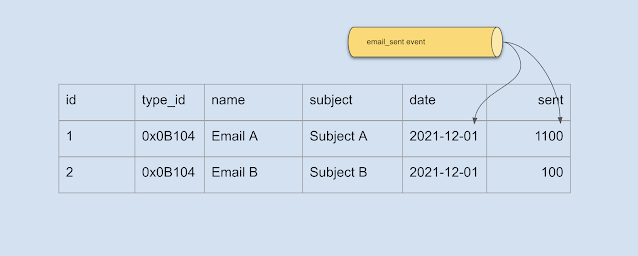
Now with the upsert implementation db.upsertRecord(message) we can achieve parity with the total number of subscribers:

id email subject date sent
1 A A 2021-12-01 13:00:00 1100
2 B B 2021-12-01 12:00:00 100

In an ideal distributed world, this would work. But immediately we can see issues. The obvious one is the loss of data overwritten by the upsert, namely the initial sent date of the A/B test for email A. Another concern would be the fact that we seem to be calculating the total for a specific record on-the-fly and updating the sent count. The other issue isn't glaringly obvious unless a failure occurs in acknowledging the message as was mentioned above. If acknowledgeEventMessage(message.Id) is invoked for the third message and fails, we could get the following state after a retry:

id email subject date sent
1 A A 2021-12-01 13:00:00 2100
2 B B 2021-12-01 12:00:00 100

What is worse is that we have no way of undoing this unless we clear the database entirely and replay the entire event stream (or at a checkpoint) which would add a lot of development hours and maintenance overhead to resolve the issue.

In order to make the system idempotent for either the case of failure or a scenario where event streams would be replayed on existing data, the original data needs to be persisted in such a way that would still benefit the normalised state of the relational database table. The following schema can help achieve this:

id email sub date_1 sent_1 date_2 sent_2 computed
1 A A ...12:00 100 ...13:00 1000 1100
2 B B ...12:00 100 (null) (null) 100

A change in table structure can help alleviate the problems of duplicate messages being consumed. It also enables persisting original data in order to avoid data loss. The unfortunate side effect however is that some records will not utilize all the data fields and will inevitably contain null values and that could be a deal breaker for the purists. Perhaps even normalizing the database table further into two separate tables with a one-to-many relationship would suffice, but that depends entirely on the volume of records and query efficiency surrounding the total sent count.

Moreover, events could be consumed out of order because there is no guarantee of order unless messages are consumed from the same partition. The above solution would still cater for this anomaly if sent_1 was 1000 and sent_2 was 100, and therefore our idempotent implementation is fulfilled.

Monday, February 10, 2020

Multiple Spark Streaming Jobs in a Single EMR Cluster


A managed Spark cluster can always save time on infrastructure maintenance. EMR (Elastic Map Reduce) is a tool that empowers data engineers to focus on building jobs to run on Spark rather than spending days managing the architecture of the cluster. However, that doesn't come without its shortfalls.

As you may already know, you can only run one job at a time in an EMR cluster. This may not be too much of an issue when running a finite Spark job or batched process since there is a completion time, however that is not the case with Spark's Structured Streaming because there is no end time!

In a self-managed vanilla Spark cluster, it is possible to submit multiple jobs to a YARN resource manager and distribute the CPU and memory allocation to share its resources even when the jobs are running Structured Streaming.

Unfortunately submitting a job to an EMR cluster that already has a job running will queue the newly submitted job. It will remain in a pending state until the previous job completes, which never does in a streaming scenario.
Having one EMR cluster for every job wouldn't be the best solution however, because AWS infrastructure costs can grow pretty quickly, especially when consulting the EMR pricing page. The main cost issues revolve around having a master node created for every EMR cluster which only passes job requests to the core nodes, and those cores may not even have their resources fully utilized for smaller streaming tasks.

This means rethinking the strategy of writing streaming jobs for use within an EMR cluster in order to work around this limitation. For this we need to look into improving the application layer.

A Typical Structured Streaming Application

The primary reason a data engineer will require the use of Structured Streaming is for consuming data from an event source, transforming it based on specific business rules or for the purpose of aggregation, and then finally persisting the result of the transformation in a data store. Typically the Scala code would require three main steps.

1. Reading from the event payload
def getEmailOpenedEvent(rawEvent: Array[Byte]): List[EmailAggregateEvent] = {
  EmailOpened.parseFrom(rawEvent)
    .map(msg =>
        EmailAggregateEvent(
          msg.getEmailId.toByteArray,
          msg.getSubscriberId.toByteArray,
          msg.getOpenedDateUtc.toTimestamp
        )
    ).toList
}
Firstly, as shown in the above code, we will need the ability to parse the payload from the event stream. The EmailOpened type is generated based on a standard byte array format (e.g. Protobuf, Avro or Thrift).

2. Transforming the messages into aggregated hourly buckets
def transformEmailOpened(ds: Dataset[EmailAggregateEvent]): Dataset[EmailAggregateData] = {
  import ds.sparkSession.implicits._

  ds.withWatermark("timestamp", "24 hours")
    .groupBy(
      col("emailId"),
      window(col("timestamp"), "1 hour")
    )
    .agg(count("*").as("eventCount"))
    .withColumn("timestampBucket", col("window.start"))
    .as[EmailAggregateData]
}
As shown above, a typical solution on how to work with streams is by aggregating the number of events based on a timestamp and maintaining an hourly bucket, which is then parsed as an EmailAggregateData type. For more information, the online programming guide on window operations in Structured Streaming can provide further detail on this type of implementation.

3. Starting the process
def process(topic: String, sql: String): Unit = {
  import spark.implicits._

  val stream = SparkSession.builder.getOrCreate
    .readEventStream(config.brokers, topic)
    .flatMap(getEmailOpenedEvent(_))

  val query = transformEmailOpened(stream)
      .writeStream
      .foreach(databaseWriter(sql))
      .trigger(Trigger.ProcessingTime("5 minutes"))
      .start

  query.awaitTermination
}
Lastly, we will need to start the process of consuming and writing to our data store. The readEventStream() function is an abstraction of SparkSession.readStream() to consume from an event source (either Apache Kafka, Amazon Kinesis, or Azure Event Hub etc). The databaseWriter() function creates a JDBC connection to execute SQL upsert commands.

There is an issue with this approach however.

If it is not already obvious, this code can quickly grow. Similar code will need to be duplicated for every event to consume from and aggregate on. Moreover, this code would require separate EMR clusters, so the code will need to be consolidated.

Consolidating repeated code using generics

Since Scala is flexible in providing a hybrid of both functional programming and Java's familiar object-oriented concepts, leveraging the use of base classes can provide great advantages.
class Event extends Product {
  // base functions
}

case class EmailAggregateEvent(
  emailId:      Array[Byte],
  subscriberId: Array[Byte],
  timestamp:    Timestamp
) extends Event {
  // override functions
}
There is one important note to consider about the above inheritance. Although Scala is flexible in enabling object-oriented programming techniques, we are still dealing with the caveats of Spark, namely serializable objects required for passing information between executors. Attempting to use a trait will actually throw an error:
Error: scala.ScalaReflectionException: <none> is not a term
This is because it simply cannot serialize a non-concrete type, and the Spark runtime is not (yet) clever enough to understand inheritance, so it will attempt to serialize the actual trait itself, which is impossible.

Moreover, when using a concrete class as the base class it will need to extend off the Product trait. This is because a case class automatically extends the Product trait which allows Spark to recognizes complex types at runtime for serialization.

Inheritance will enable us to achieve the following:
case class Job[T >: Event, U >: Data](
    topic:     String,
    consume:   Array[Byte] => List[T],
    transform: Dataset[T] => Dataset[U],
    sql:       String
)
The Job type can now help substitute any job-specific implementation in the process() function as follows:
def process[T >: Event, U >: Data](job: Job[T, U]): Unit = {
  import spark.implicits._

  val stream = SparkSession.builder.getOrCreate
    .readEventStream(config.brokers, job.topic)
    .flatMap(job.consume(_))

  val query = job.transform(stream)
      .writeStream
      .foreach(databaseWriter(job.sql))
      .trigger(Trigger.ProcessingTime("5 minutes")))
      .start

  query.awaitTermination
}
Unfortunately this will still not be enough.

In the original transformEmailOpened() function above, there are implicit conversions which can no longer work when using inheritance. The Spark API provides an easy to use property called as[T] which returns a new Dataset where each field is mapped to columns of the same name of the given type T. During runtime Spark will need a little help to understand what type is required explicitly, so the transformEmailOpened() function will need to change as follows:
def transformEmailOpened(ds: Dataset[EmailAggregateEvent]): Dataset[EmailAggregateData] = {
  import ds.sparkSession.implicits._

  ds
    // explicitly map to concrete type
    .map(row => EmailAggregateEvent(
      row.emailId,
      row.subscriberId,
      row.timestamp
    ))
    .withWatermark("timestamp", "24 hours")
    .groupBy(
      col("emailId"),
      window(col("timestamp"), "1 hour")
    )
    .agg(count("*").as("eventCount"))
    .withColumn("timestampBucket", col("window.start"))
    // replace as[T] with explicit map
    .map(row => EmailAggregateData(
      row.getAs("emailId"),
      row.getAs("timestampBucket"),
      row.getAs("eventCount")
    ))
}
Inheritance can now work at runtime, and will enable our code to scale when more events are required for consumption. Adding multiple jobs can now be relatively easy.

However, we cannot simply just write a jobs.foreach() implementation and expect it to work since it will never iterate past the first streaming job. This is where concurrency plays an important role in the overall solution.

Concurrency

Enabling parallel programming in Scala is very simple. The .par() function enables parallel processing of a collection in an extremely concise way. We can take advantage of this by wrapping the entire functionality of the process() function into a parallel foreach() loop as follows:
jobs.par.foreach(job => {
  process(job)
})
There is one thing that hasn't been considered with the above code though. The SparkSession that is used within the process() function is a static object and only one can be active per Spark cluster. However that doesn't mean we cannot start multiple streaming jobs using the same SparkSession! The SparkSession.readEventStream() functionality won't be a problem running in parallel even though the function is being called multiple times against the same static Spark session.

In terms of concurrency though, the .par() functionality is a multi-threaded implementation. In the JVM framework each thread runs on one CPU unit (either a physical processor or hyper-threaded processor). This means a multi-threaded approach would only work if the number of jobs required is less than the number of processors in the EMR cluster. To find out how many cores (and essentially how many separate threads the job can run on) the following value can be outputted:
Runtime.getRuntime.availableProcessors
The problem with this solution is cost. When considering that each job may only utilize 5% or less of the CPU units, we may have more cores in the EMR cluster than is necessary. As an example, running 12 jobs concurrently means the next instance size up to support this is m4.4xlarge which has 16 cores. That is a total of 4 cores that will sit idle never to be used. Moreover, each used core may also be underutilized.

Considering asynchronous programming rather than a multi-threaded approach suddenly becomes more relevant, and Scala's Futures can come in handy with only a few simple changes:
val executionContext = ExecutionContext.fromExecutorService(Executors.newFixedThreadPool(maxConcurrentJobs))

val tasks: List[Future[Unit]] = jobs
  .map(job =>
    Future {
      process(job)
    }(executionContext)
  )

Await.result(Future.sequence(tasks)(implicitly, executionContext), Duration.Inf)
With this minimal code change we can have massive benefits in cost reduction. By default the thread pool count (i.e. the maximum number of concurrent runs) is actually the number of processors, just like the multi-threading approach. This is where the executionContext comes in handy to explicitly set the number of concurrent executions with the maxConcurrentJobs variable. This number can be as large as necessary to handle as many job across the entire EMR cluster regardless of how many cores are provisioned. The limit can now be based on the exact number of cores and the resource allocation required per individual job.

Conclusion

Even with the limitations of EMR clusters allowing only one job to run at any given time, as well as considering that only one static SparkSession object exists per Spark job, there are still efficient ways to work around these limitations.

Jobs can be refactored to enable consolidation of code repetition which in turn enables the possibilities of concurrent processing. This can significantly reduce cost of infrastructure and keep a clean code base that can be extensible.

Thursday, January 10, 2019

Compiling Spark Jobs using SBT on Build Machines

Deploying a Spark job can be challenging, especially considering that one Spark job is never the same as another. Deployment times can vary significantly depending on a wide range of factors. Finding ways to make the deployment efficient can greatly improve the process, and that can be achieved with a few simple strategies.

Consider the following steps required to deploy a Spark job that is built in scala and compiled using sbt:
  1. Get latest project files (requires git or subversion etc.)
  2. Download dependencies (requires sbt)
  3. Compile Spark application (requires sbt)
  4. Run unit test (requires sbt)
  5. Package Spark application to a .jar file (requires sbt)
  6. Upload .jar file to an accessible location (e.g. s3 bucket) (requires aws-cli)
  7. Spark submit using the s3 location to the master node (requires spark)
This can be achieved using a deployment pipeline created in a CI tool like TeamCity or Jenkins.
Usually build machines used for a deployment pipeline are provisioned so they are lightweight with very few applications installed.
In fact, if the only application installed on a build machine is docker, then that is enough.

Since our build machines don't have sbt installed, a docker image with scala and sbt is required to run sbt assembly. A docker image found on docker hub like spikerlabs/scala-sbt can achieve this. However, running sbt assembly using this docker image will take a significantly long time to complete, sometimes as long as 30 minutes! This is because all the necessary dependencies for your spark job will need to be downloaded before compiling your Spark application.

Performing this operation every time you need to deploy your Spark job is costly. So in order to improve the efficiency of builds to prevent these download times, the dependencies first need to be downloaded onto a specific sbt docker image that is tailored for your Spark job. This can then be used as part of the deployment pipeline.

The following steps will need to be carried out for this to be achieved:

1. cd into the project folder.

2. Run the following docker command to start a spikerlabs/scala-sbt container in interactive mode.
docker run -i -v "/$(pwd)/":/app -w "//app" --name "my-scala-sbt-container" "spikerlabs/scala-sbt:scala-2.11.8-sbt-0.13.15" bash
Note that a specific scala and sbt version will alway be required otherwise the "latest" tag could fail during compilation with any breaking changes.

3. Once in interactive mode within the docker container, run the following commands within the container.
> sbt assembly # to download dependencies, compile, and package the spark job
> exit # once the packaging is complete
4. This will create a docker container called my-scala-sbt-container which will need to be exported, then imported as an image, as follows:
docker export --output="./my-scala-sbt-container.tar" "my-scala-sbt-container"
docker import "./my-scala-sbt-container.tar" [INTERNAL_REPOSITORY_URL]/my-scala-sbt-image:[VERSION_NUMBER]
Where [INTERNAL_REPOSITORY_URL] is a company wide docker repository location e.g. like nexus,
and where [VERSION_NUMBER] needs to be bumped up from a previous version.

Note that the import allows a container that has all the necessary dependencies to be converted into an image called [INTERNAL_REPOSITORY_URL]/my-scala-sbt-image:[VERSION_NUMBER].

This will be needed when docker push is executed. Unfortunately the docker API for a push command requires the image name to be exactly the same as the docker repository url which seems a little non-intuitive.

5. To publish the the local docker image to the internal docker repository, run the following docker push command:
docker image push [INTERNAL_REPOSITORY_URL]/my-scala-sbt-image:[VERSION_NUMBER]
Where [INTERNAL_REPOSITORY_URL] is a company wide docker repository location e.g. like nexus,
and where [VERSION_NUMBER] is the same as the previous step.

This can now help in the CI deployment pipeline, where the step to run sbt assembly can be done with the docker run command as follows:
cat <<EOF > assembly.sh
    
#!/usr/bin/env bash
set -ex
sbt assembly
EOF docker run \ --rm \ -v "/$(pwd)/..":/app \ -v "/$(pwd)/assembly.sh":/assembly.sh \ -w "//" \ --entrypoint=sh \ [INTERNAL_REPOSITORY_URL]/my-scala-sbt-image:[VERSION_NUMBER] \ //assembly.sh
That should improve the build timings by removing up to 30 minutes off the deployment pipeline, depending on how many dependencies are required for the Spark application.

Wednesday, September 26, 2018

Automating Deployments for Spark Streaming on AWS EMR

Anyone who's familiar with submitting a Spark job will know it's as simple as running a single command, so long as the Spark CLI is installed on the machine running that command:
spark-submit --master ${MASTER_ENDPOINT} --deploy-mode cluster --class com.cm.spark.SparkApp s3://bucket/jobs/${APP_JAR}
Elastic Map Reduce

This is easy enough when working with a self-managed vanilla Spark cluster. AWS also provides a service called EMR (Elastic Map-Reduce) which offers hosting of Spark clusters and so the AWS CLI provides an equally effortless way to submit Spark jobs:
aws emr add-steps cluster-id j-UJODR7SZ6L7L steps Type=Spark,Name="Aggregator",ActionOnFailure=CONTINUE,Args=[--deploy-mode,cluster,--class,com.cm.spark.SparkApp,s3://bucket/jobs/${APP_JAR}]
This is essentially a wrapper around the spark-submit command. The AWS documentation is relatively detailed in providing information for adding additional parameters to the command line arguments in order to provide all the features found in the spark-submit command. This makes it incredibly simple to create a deployment step in your CI pipeline.

Even if the build machines don't have AWS CLI installed, the commands can be wrapped around a docker run call using an image called garland/aws-cli-docker which can be found on Docker Hub:
cat <<EOF > submit.sh

    #!/usr/bin/env bash

    set -ex

    aws emr add-steps cluster-id j-UJODR7SZ6L7L steps ...
    
EOF

docker run \
    --rm \
    -e AWS_DEFAULT_REGION=${AWS_REGION} \
    -e AWS_ACCESS_KEY_ID="${AWS_ACCESS_KEY_ID}" \
    -e AWS_SECRET_ACCESS_KEY="${AWS_SECRET_ACCESS_KEY}" \
    -v "/${APP_JAR}":/${APP_JAR} \
    -v "/$(pwd)/submit.sh":/submit.sh \
    -w "//" \
    --entrypoint=sh \
    garland/aws-cli-docker:latest \
    //submit.sh
The beautiful thing about docker is that the build machines only ever need one prerequisite: docker. Anything else that needs to be installed for deployment can instead be found as a docker image on Docker Hub. In this case the aws emr add-steps command is executed within a docker container and the build machines don't need to know anything about it!

However, there is a catch. This is only straightforward if you are under the assumption that your Spark job eventually completes, whether it returns a success or failure status. In fact, that is exactly the same assumption that the AWS documentation makes. Once a job completes, running the same command will add a new step on the cluster and the step will run without any issues.

But what about Structured Streaming? An ongoing Spark job with an open connection to listen to an event stream suddenly makes one simple command slightly more complicated when deployment of a code change is required.

This would require stopping a currently running step before adding a new step. AWS documentation has another command that can be useful in this scenario:
aws emr cancel-steps --cluster-id j-UJODR7SZ6L7L --step-ids s-2V57YI7T5NF42
Unfortunately the cancel-steps command can only remove a pending step i.e. one that isn't in a running state. In fact there is no API to terminate a running step at all and the only solution found in AWS documentation is to do the following:
  1. Log into the EMR master node (which will need a secure .pem file)
  2. Run yarn application -list
  3. Find the application ID of the currently running job
  4. Run yarn application -kill ${APP_ID}
Obviously this is not a viable solution for automation since we will have to deal with ssh and passing .pem files around on build machines in order to achieve this process. No doubt your security team would have their own opinion on this approach.

Alternatively, there is another AWS API call that may be a useful workaround:
aws emr terminate-clusters --cluster-ids j-UJODR7SZ6L7L
This could achieve what we are looking for, if the following automation steps are executed:
  1. Terminate EMR cluster
  2. Recreate EMR cluster using terraform or cloud formation
  3. Add step to newly created cluster
Terminating an entire cluster just to deploy a job may seem like overkill, however in the new world of infrastructure-as-code, it isn't quite as insane as one might think. After consulting AWS experts and Spark specialists alike, both have agreed that these days it is actually encouraged to dedicate one spark job to a single Spark cluster.

The benefits are quite significant:
  • Dedicated clusters mean each job can only affect itself without consuming resources from other jobs
  • If there are any fatal errors or memory leaks other jobs aren't affected
  • The entire cluster's resources can be specifically tailored for a single job, rather than maintaining resource allocation for many jobs which will require significant monitoring and any necessary resizing will affect all currently running jobs with downtime
However, the downfalls are also notable:
  • Rather than one single master with many shared cores, there will be a master for each job which will obviously mean more EC2 costs, however masters can be kept small since they're only required to receive requests and distribute compute to slaves
  • Deployment pipelines will be slower since recreating clusters for every application code update will add significant time to the build process
These downfalls may be deal breakers for some use cases, and it has given enough attention to the AWS experts after consultation to at least rethink the API strategies they've provided for a scenario such as Structured Streaming. The initial assumption that a Spark job is a short lived process is simply not enough.

A better solution for now would actually be to utilise the YARN API instead. Since YARN is the orchestrator of the Spark nodes within the cluster, it provides many features in which to manage both the cluster and its jobs. There is comprehensive documentation on every command available via HTTP REST API calls. That means the build machines can avoid having to ssh into master nodes using .pem files and can send an HTTP request instead (so long as the inbound firewall permissions of the Spark cluster allow the build machines access to it - and that is a simple terraform or cloud formation configuration).

That means the following automation steps can achieve a successful deployment pipeline:
# 1. Get a list of active jobs
APPS=$(curl -s -X GET -H "Content-Type: application/json" "http://${MASTER_ENDPOINT}/ws/v1/cluster/apps")

# 2. Parse the response payload and return the id of the running job (requires jp package)
APP_ID=$(echo $APPS | jq '.apps.app[0].id')

# 3. Send a kill request to the currently running job
curl -X PUT -H "Content-Type: application/json" -d '{"state": "KILLED"}' "http://${MASTER_ENDPOINT}/ws/v1/cluster/apps/${APP_ID}/state"

# 4. Add a new step to submit the new job
aws emr add-steps cluster-id j-UJODR7SZ6L7L steps Type=Spark,Name="Aggregator",ActionOnFailure=CONTINUE,Args=[--deploy-mode,cluster,--class,com.cm.spark.SparkApp,s3://bucket/jobs/${APP_JAR}]
This removes all the downfalls because it creates a separation of concerns by providing a specific CI pipeline for job deployment while the cluster can be resized and rebuilt when necessary. The benefits of keeping one dedicated cluster per Spark job can still be maintained with this solution, only that the cluster doesn't have to be destroyed every time there is an iteration required on the job itself.

Monday, October 30, 2017

Aggregating Event Streams in Redshift using Matillion

If you haven’t heard of Matillion, then it’s time you knew about it. If you’ve used ETL tools in the past like the traditional SSIS for Microsoft’s SQL Server, then Matillion would be very familiar to you. Where SSIS was tailored for SQL Server, Matillion is tailored for Amazon’s Data Warehouse offering, AWS Redshift.


Matillion’s user interface is very intuitive as it groups all its components into three natural categories: those for extract, those for transform, and those for load.

Since Matillion sits on top of Redshift, both must live within AWS, so the features for extracting include components for RDS (as well as any other relational databases that support JDBC drivers). It also supports DynamoDB, S3, as well as components for MongoDB, Cassandra and Couchbase.


Components used for transformation provide the ability to aggregate, filter, rank, and even to roll up sums over multiple records from a transient “staging” Redshift table to load it to a more permanent Redshift table. The underlying functions for these components are in fact Redshift query commands.

Matillion seems quite mature with countless component features at your fingertips. Much of the transformation logic you can construct can definitely be written by hand using Redshift’s comprehensive documentation on ANSI SQL commands, but what Matillion can provide is a visual representation which significantly improves collaboration amongst team members so they can all be equally responsible for maintaining the ETL process in an efficient way.

Many could be forgiven for associating an ETL process with the old techniques of extracting large amounts of data from a monolithic data store to push into a read store using the typical CQRS architecture, but Matillion can be used for much more than that.

Our use-case at Campaign Monitor not only required data from a snapshot-style structure as is found in a traditional monolithic relational database, but also data that is sourced from an event stream for a rolling daily aggregation.

In order to achieve this we needed an initial query to obtain the total snapshot on a particular day, which can then be stored in a “roll-up” table in Redshift as the first day of aggregated totals. Let’s take the following table as an example snapshot that can be the baseline for any future events:

ListIDSubscribersDate
110002017-10-01
220002017-10-01
330002017-10-01
440002017-10-01

This can be done using a traditional ETL job in Matillion as follows:


There is a lot of sophisticated magic under the hood with regards to the Database Query component. The SQL query that is run from the relational database will return a resultset that Matillion can chunk into separate concurrent processes. Each of these processes will create an underlying S3 file before loading the data into the “rs_lists_subscriber_rollup_staging” table in Redshift.

Once we have a snapshot on a particular date (in this case 2017–10–01 in the example above) all events for subscribers that come in after this date can be streamed from our event source, and then aggregated into the same table with a rolling count of subscribers for subsequent dates.

This requires some form of consumption externally to receive the incoming events, which can be batched into S3 files, and then persisted into an ephemeral “raw” table in Redshift using the COPY command. This raw table would look as follows:

ListIDSubscriberIDSubscribe TallyDate
1112017-10-02
12-12017-10-02
3112017-10-02
2112017-10-02
2212017-10-02
2312017-10-02
41-12017-10-02
42-12017-10-02
43-12017-10-02
4412017-10-02
4112017-10-03
4512017-10-03
4612017-10-03
4712017-10-03

Generally, a contact subscribes or unsubscribes at a specific time from a list, and this will need to be aggregated daily per list so the data above would look as follows:

ListIDSubscribersDate
102017-10-02
232017-10-02
312017-10-02
4-22017-10-02
442017-10-03

This aggregation can also be done in Matillion very easily from the raw table:


The Aggregate component would simply need to sum the Subscribe/Unsubscribe column with a grouping of ListID. Once this is achieved, there will need to be a union of data from the existing snapshot data so that there can be a baseline to work with for rolling counts. Only then can the very powerful Window Calculation component be used for rolling up the sum of subscribers based on a partition (in this case the ListID) and a partition ordering (in this case Date). The Matillion job would look as follows:


There are further properties for the Windows Calculation component that need to be considered, including setting the lower bound to “unbounded preceding”. This ensures that the calculated sum is rolled up from the very first record of the dataset that was unioned from the previous component. The properties would look as follows:


There are of course other edge cases that will need to be considered that could slowly make your transformation job increasingly complex. These can include lists that were created after the snapshot was taken, or even more interesting is catering for missing days that receive no events which will need to be populated with a default of zero so aggregation can be included in the roll-up for that day. Thankfully Matillion makes it simple to grow on the above transformation so it can be easily maintained.

The final table would then look as follows:

ListIDSubscribersDate
110002017-10-01
220002017-10-01
330002017-10-01
440002017-10-01
110002017-10-02
220032017-10-02
330012017-10-02
439982017-10-02
110002017-10-03
220032017-10-03
330012017-10-03
440022017-10-03

And this can then be used when reporting over date ranges from your front end reporting application.

This example is just one of many use-cases where Matillion has helped Campaign Monitor fulfill its ETL requirements in order to provide reporting on large datasets. In particular, event based data has helped significantly improve SLAs since the frequency of aggregating data can be done within minutes compared to that of the traditional relational data ETLs that process large queries over many hours and provide much lower refresh rates for report data.

Wednesday, September 13, 2017

Gotchas with Altering Table Schemas in Redshift

As I learned recently the hard way, simply altering tables in Redshift to perform a simple operation of adding columns doesn't behave the same way in a data warehouse as it does in regular relational databases.

Running the following SQL statement in Redshift actually has a lot more issues than you would expect:

ALTER TABLE rs_table ADD COLUMN new_column;

Despite the simple nature of this statement, many issues begin to emerge.

One of these is table locking. If an application is connecting to it via JDBC, connections would end up being queued because one Redshift cluster only allows 500 concurrent connections as per their online documentation.

Moreover, it was noticed that there were a number of duplicate records when inserts occurred on a matching key instead of updating the existing record or deleting the old record. This was most likely due to the fact that it was in the process of being altered during an insert and the key match could not be found.

This meant that an alternative approach was needed in order to prevent the locking and concurrency.
The following steps were tried and tested, and proved to work well:
  • Create the new table with the new schema suffixed with _new
  • Copy data from the old table to the new table
  • Rename old table suffixed with _old
  • Rename new table removing _new suffix
This is done in SQL as follows:

-- Create new table with new schema
CREATE TABLE rs_table_new
(
    id numeric(10),
    name varchar(250),
    date timestamp,
    new_column numeric(10)
) SORTKEY(dbid, date, clientid);
-- Copy data from old table to new
INSERT INTO rs_table_new
SELECT
    id,
    name,
    date,
    NULL
FROM rs_table;
-- Rename table
ALTER TABLE rs_table RENAME TO rs_table_old;
ALTER TABLE rs_table_new RENAME TO rs_table;

Amazingly, the total execution time for a table with over 10 million records completed in under 2 minutes as opposed to the initial 2 hours.

Monday, June 13, 2016

Don't Always Believe Your Data

As erroneous as that statement might seem, not trusting your data might be the most prudent thing you do. In this new age of data-driven development where data has become a precious commodity, the need to unlock valuable information that businesses hold about customer interactions has become a crucial part of business success, and hence the investment for better ways to store and extract data has evolved over the last few years more than it ever had over the previous two decades.

The options are endless now with experts recommending vast arrays of strategies to tackle your storage and analysis techniques. But it is more than just the sum of all knowledge about these alternatives that makes you a Data Scientist. The reason we store data in the first place is to provide information that can remove ambiguity in our decision making process. That requires a broader outlook towards investigating industry trends and changes in technology on top of our expertise on how well we persist and describe our business data.

There was a time when relational data stores ruled the earth and with them came the ability to analyse large amounts of data using OLAP cubes. But as the need grew for a more efficient Extract Transform Load (ETL) process the limitations became obvious. Analyzing records that were aggregated nightly because there was “too much data” to extract no longer became a legitimate excuse. Businesses want it now, and they want a lot of it.

With that, storage capabilities evolved to scale horizontally with the map-reduce patterns of document stores like Mongo, key-value stores like Riak, graph stores like Neo4j, and columnar stores like Cassandra. Add into the mix the likes of Big Data storage such as Hadoop, and Event Streams for real time processing like kafka and Amazon Kinesis. Although competition is always a welcome dynamic in any industry, with every contender vying for feature capabilities over their competitors, the choice becomes difficult.

Storage is just one part of the puzzle however. Next would come analysis and forecast. Once a business makes sense of the data it holds with a myriad of techniques for analysis, predicting change comes packaged for us with Machine Learning. Apache Spark jumped on this wagon early commercially with its MLlib offering and Google has also been a popular choice with TensorFlow. There is a degree of expertise required in handling these tools including understanding the type of learning you want your machine to perform, whether its supervised learning using labeled datasets (for fraud detection and recommendations), unsupervised and semi-supervised learning with unlabeled datasets (for image and voice recognition), or reinforcement learning (for artificial intelligence).

There is more to it than knowing your alternatives though. Your data can only tell you as much information as your business keeps about itself, and so Data Science is not just about how to unlock your data with the available tools, its about causation. It's about why.

Identifying peaks or troughs in a graph might help you determine with a guarantee that your tools can help you see patterns or changes, but not the reasons why these patterns and changes exist. And thus starts the real investigation.

This was a lesson that Andrea Burbank from Pinterest learnt as she explained at the YOW! Conference held in Sydney late 2016, and she was kind enough to share her challenges in trying to successfully formulate behavioral trends from Pinterest's massive data storage. The results of her findings were very interesting.

By measuring "daily active users", Pinterest were able to determine which unique customers engaged on their site. Using kafka, they were able to stream logs of response data that told the user's story, but that was just basic counting.

In late October of 2013, they found a sudden step change in growth rate specifically with iPhone users, which seemed likely to be the result of Pinterest being featured in the App Store. What they found though was that it was merely a coincidence because not long before a new feature was introduced to iOS 7 called "Background App Refresh" to prevent apps hanging in suspended animation.

Burbank realized that the statistics they generated weren't telling the full story and after digging further found that one of their endpoints, particularly the home feed endpoint, was giving unnatural background hits even when the app wasn't appearing in the multitask tray, and that obviously had no correlation to daily active users.

This lead to what Burbank defined as the "Spectrum of Certainty" where correlation is found at one end of the spectrum while causation is found at the other. Most of the time Data Scientists believe they are closer to the causation end of the spectrum, when in actual fact they sit very close to the correlation side.

The goal is to ensure data analysis moves towards causal inference, in effect requiring much more investigative techniques about events that occur outside the business domain which may have a strong impact on how data is represented within the business itself. Only then can you truly believe your data to a certain degree.

Reference: Data science as software, Andrea Burbank, Pinterest, YOW! Conference 2016 Sydney

Friday, December 18, 2015

INNER JOIN vs WHERE EXISTS Sub-Queries in MSSQL

Currently working at WiseTech, I've learn't a great deal about the pros and cons of monolithic applications, and more so about why microservices have been a massive talking point in the industry today. There are many specialists in the technology stack here and recently I got into a discussion about SQL performance tuning.

For a long time I always thought there was a standard golden rule when it came to arguing against sub-queries, and it was almost as sacrilege as cursors, however there have been a few circumstances where the difference may actually vary very little.

Here is a very simple statement that contains one INNER JOIN:

SELECT *
FROM StmNote
INNER JOIN JobDeclaration ON JE_PK = ST_ParentID
WHERE ST_Description = 'Justification Note'
       AND ST_Table <> 'JobDeclaration';

And below is an identical query that returns the same results, only with the difference being that it contains a WHERE EXISTS sub-query clause instead of an INNER JOIN:

SELECT *
FROM StmNote
WHERE ST_Description = 'Justification Note'
       AND ST_Table <> 'JobDeclaration'
       AND EXISTS (SELECT 1 FROM JobDeclaration WHERE JE_PK = ST_ParentID);

The below execution plan proves there is absolutely no difference in the decision path that the query optimizer makes.


This could easily make one argue that the difference in both statements would simply come down to a matter of preference.

However as we know the query optimizer behaves very differently when considering the number of rows involved in an index-seek/table-scan and the statistics it has to work with in determining and efficient execution path.

So what if there were other joins or larger result sets which could ultimately mean more variations in the execution path for query optimizer?

Below is a more complex scenario involving multiple joins that in the first case uses the following query:

SELECT bna.*
FROM BmncnAttachment bna
INNER JOIN BmncnShape bns
       ON bns.BNS_PK = bna.BNA_BNS_FromShape OR bns.BNS_PK = bna.BNA_BNS_ToShape OR bns.BNS_PK = bna.BNA_BNS_Owner
INNER JOIN ProcessHeader fh
       ON bns.BNS_FH_ProcessHeader = fh.FH_PK
INNER JOIN WorkItem wki
       ON wki.WKI_PK IS NOT NULL
WHERE wki.WKI_PK = fh.FH_ParentId
       AND wki.WKI_Summary LIKE 'Issue %'
       AND wki.WKI_Status IN ('ASN', 'OPN', '');

While the second case uses the following query with a WHERE EXISTS sub-query clause:

SELECT bna.*
FROM BmncnAttachment bna
INNER JOIN BmncnShape bns
       ON bns.BNS_PK = bna.BNA_BNS_FromShape OR bns.BNS_PK = bna.BNA_BNS_ToShape OR bns.BNS_PK = bna.BNA_BNS_Owner
INNER JOIN WorkItem wki
       ON wki.WKI_PK IS NOT NULL
WHERE wki.WKI_Summary LIKE 'Issue %'
       AND wki.WKI_Status IN ('ASN', 'OPN', '')
       AND EXISTS (SELECT 1 FROM ProcessHeader fh WHERE bns.BNS_FH_ProcessHeader = fh.FH_PK AND wki.WKI_PK = fh.FH_ParentId);

And here is the varying execution plans for both:


It seems they differ significantly on the final Hash Matching where it is probing the hash key fh.FH_ParentId and taking 62% or the total time longer than the standard inner join. The is mainly because you lose parallelism when using the sub-query.

So basically to sum it all up, even though the first statement may show identical results, performance issues would exists if there were multiple joins, because the optimizer could choose the sub-query over another join which would otherwise have been more efficient.

Conversely however, performance could be effected for joins that return duplicate rows and that may be another variable to consider when making the decision between WHERE EXIST sub-query clauses and JOINS, and is definitely something to keep in mind when making the final decision on what type of statement to use.